The search for a substring in a string is carried out according to a given pattern, i.e. some sequence of characters whose length does not exceed the length of the original string. The job of a search is to determine whether a string contains a given pattern and to indicate the location (index) in the string if a match is found.
The brute force algorithm is the simplest and slowest and consists of checking all text positions to see if they match the beginning of the pattern. If the beginning of the pattern coincides, then the next letter in the sample and in the text is compared, and so on, with the most recent simple and slowest answer, whether there is such an element or not, without indicating whether it is already sorted by the lack of complete match of the pattern or the difference in the next letter.
int BFSearch(char *s, char *p)
for (int i = 1; strlen(s) - strlen(p); i++)
for (int j = 1; strlen(p); j++)
if (p[j] != s)
if (j = strlen(p))
The BFSearch function searches for the substring p in the string s and returns the index of the first character of the substring or 0 if the substring is not found. Although this method, like most brute force methods, is generally ineffective, in some situations it is quite acceptable.
Fastest among algorithms general purpose, designed to search for a substring in a string, is considered the Boyer-Moore algorithm, developed by two scientists - Boyer (Robert S. Boyer) and Moore (J. Strother Moore), the essence of which is as follows.
Boyer-Moore algorithm
The simplest option Boyer-Moore algorithm consists of next steps. The first step is to build a table of displacements for the desired sample. The table construction process will be described below. Next, the beginning of the line and the sample are combined and the check begins with last character sample. If the last character of the pattern and the corresponding character of the line when superimposed do not match, the pattern is shifted relative to the line by the amount obtained from the offset table, and the comparison is performed again, starting from the last character of the pattern. If the characters match, the penultimate character of the sample is compared, and so on. If all the characters in the pattern match the superimposed characters in the string, then the substring has been found and the search is over. If some (not the last) character of the pattern does not match the corresponding character of the string, we shift the pattern one character to the right and start checking again from the last character. The entire algorithm is executed until either an occurrence of the desired pattern is found or the end of the string is reached.
The amount of shift in case of a mismatch of the last character is calculated according to the rule: the shift of the pattern must be minimal, so as not to miss the occurrence of the pattern in the line. If a given string character occurs in a pattern, the pattern is shifted so that the string character matches the rightmost occurrence of that character in the pattern. If the pattern does not contain this character at all, then the pattern is shifted by an amount equal to its length, so that the first character of the pattern is superimposed on the next character of the line being tested.
The offset value for each character of the pattern depends only on the order of the characters in the pattern, so it is convenient to calculate the offsets in advance and store them in the form of a one-dimensional array, where each character of the alphabet corresponds to an offset relative to the last character of the pattern. Let us explain all of the above in simple example. Let there be a set of five characters: a, b, c, d, e, and you need to find an occurrence of the pattern “abbad” in the string “abecccacbadbabbad”. The following diagrams illustrate all stages of the algorithm:
Displacement table for the “abbad” sample.
Start the search. The last character of the pattern does not match the overlay character of the string. Shift the sample to the right by 5 positions:
Three of the sample symbols matched, but the fourth did not. Shift the sample to the right one position:
The last character again does not match the character of the string. In accordance with the displacement table, we shift the sample by 2 positions:
Once again we shift the sample by 2 positions:
Now, in accordance with the table, we shift the pattern by one position and get the desired occurrence of the pattern:
Let's implement the specified algorithm. First of all, you need to define the offset table data type. For a code table consisting of 256 characters, the structure definition will look like this:
BMTable MakeBMTable(char *p)
for (i = 0; i<= 255; i++) bmt->bmtarr[i] = strlen(p);
for (i = strlen(p); i<= 1; i--)
if (bmt->bmtarr] == strlen(p))
bmt->bmtarr] = strlen(p)-i;
Now let's write a function that performs a search.
int BMSearch(int startpos, char *s, char *p)
pos = startpos + lp - 1;
while (pos< strlen(s))
if (p != s) pos = pos + bmt->bmtarr];
for (i = lp - 1; i<= 1; i--)
if (p[i] != s)
return(pos - lp + 1);
The BMSearch function returns the position of the first character of the first occurrence of pattern p in string s. If the sequence p in s is not found, the function returns 0. The startpos parameter allows you to specify the position in string s at which to start the search. This can be useful if you want to find all occurrences of p in s. To search from the very beginning of the string, set startpos to 1. If the search result is non-zero, then to find the next occurrence of p in s, set startpos to the value “previous result plus pattern length.”
Binary (binary) search
Binary search is used when the array being searched is already ordered.
The variables lb and ub contain, respectively, the left and right boundaries of the array segment where the desired element is located. The search always begins with an examination of the middle element of the segment. If the desired value is less than the middle element, then you need to move on to searching in the upper half of the segment, where all elements are less than the one just checked. In other words, the value of ub becomes (m – 1) and in the next iteration half of the original array is checked. Thus, as a result of each check, the search area is narrowed by half. For example, if there are 100 numbers in the array, then after the first iteration the search area is reduced to 50 numbers, after the second to 25, after the third to 13, after the fourth to 7, etc. If the length of the array is n, then about log 2 n comparisons are enough to search the array of elements.
Brute Force Method
Complete search(or brute force method from English brute force) - a method of solving a problem by searching through all possible options. The complexity of a complete search depends on the dimension of the space of all possible solutions to the problem. If the solution space is very large, then exhaustive search may not yield results for several years or even centuries.
See what the “Brute Force Method” is in other dictionaries:
Complete search (or the “brute force” method from the English brute force) is a method of solving a problem by searching through all possible options. The complexity of a complete search depends on the dimension of the space of all possible solutions to the problem. If the solution space... ... Wikipedia
Sorting by simple exchanges, bubble sort is a simple sorting algorithm. This algorithm is the simplest to understand and implement, but it is effective only for small arrays. Algorithm complexity: O(n²). Algorithm... ... Wikipedia
This term has other meanings, see Overkill. Brute force (or brute force) is a method for solving mathematical problems. Belongs to the class of methods for finding a solution by exhausting all possible... ... Wikipedia
Cover of the first edition of the brochure “Bail's Papers...” Bale's cryptograms are three encrypted messages, as expected, containing information about the location of a treasure of gold, silver and precious stones, allegedly buried on the territory ... Wikipedia
Snefru is a cryptographic one-way hash function proposed by Ralph Merkle. (The name Snefru itself, continuing the traditions of the block ciphers Khufu and Khafre, also developed by Ralph Merkle, is the name of the Egyptian ... ... Wikipedia
An attempt to crack (decrypt) data encrypted with a block cipher. All major types of attacks apply to block ciphers, but there are some attacks that are specific only to block ciphers. Contents 1 Types of attacks 1.1 General ... Wikipedia
Neurocryptography is a branch of cryptography that studies the use of stochastic algorithms, in particular neural networks, for encryption and cryptanalysis. Contents 1 Definition 2 Application ... Wikipedia
The optimal route for a traveling salesman through the 15 largest cities in Germany. The indicated route is the shortest of all possible 43,589,145,600. Traveling salesman problem (TSP) (traveling salesman ... Wikipedia
Cryptographic hash function Name N Hash Created 1990 Published 1990 Hash size 128 bits Number of rounds 12 or 15 Type of hash function N Hash cryptographic ... Wikipedia
The traveling salesman problem (traveling salesman) is one of the most famous combinatorial optimization problems. The task is to find the most profitable route passing through the specified cities at least once every... ... Wikipedia
The brute force method is a direct approach to solving
of a problem, usually based directly on the problem statement and definitions of the concepts it uses.
A brute force algorithm for solving a general search problem is called sequential search. This algorithm simply compares the elements of a given list with the search key one by one until an element with the specified key value is found (successful search) or the entire list is checked but the desired element is not found (failed search). A simple additional trick is often used: if you add the search key to the end of the list, the search will definitely be successful, therefore, you can remove the check for list completion in each iteration of the algorithm. The following is the pseudocode for such an improved version; it is assumed that the input data is in the form of an array.
If the original list is sorted, you can take advantage of another improvement: the search in such a list can be stopped as soon as an element is encountered that is no smaller than the search key. Sequential search provides an excellent illustration of the brute force method, with its characteristic strengths (simplicity) and weaknesses (low efficiency).
It is quite obvious that the running time of this algorithm can vary within very wide limits for the same list of size n. In the worst case, i.e. when the list does not contain the desired element, or when the desired element is located last in the list, the algorithm will perform the largest number of operations comparing the key with all n elements of the list: C(n) = n.
1.2. Rabin's algorithm.
Rabin's algorithm is a modification of the linear algorithm, it is based on a very simple idea:
“Let's imagine that in a word A, the length of which is m, we are looking for a pattern X of length n. Let's cut out a "window" of size n and move it along the input word. We are interested in whether the word in the “box” matches the given pattern. It takes a long time to compare letters. Instead, we fix some numerical function on words of length n, then the problem will be reduced to comparing numbers, which is undoubtedly faster. If the values of this function on the word in the “box” and on the sample are different, then there is no coincidence. Only if the values are the same, it is necessary to check the letter-by-letter match sequentially.”
This algorithm performs a linear traversal over a line (n steps) and a linear traversal over the entire text (m steps), so the total running time is O(n+m). At the same time, we do not take into account the time complexity of calculating the hash function, since the essence of the algorithm is that this function should be so easy to calculate that its operation does not affect the overall operation of the algorithm.
Rabin's algorithm and the sequential search algorithm are the least labor intensive algorithms, so they are suitable for use in solving a certain class of problems. However, these algorithms are not the most optimal.
1.3. Knuth-Morris-Pratt (kmp) algorithm.
The KMP method uses preprocessing of the search string, namely: a prefix function is created on its basis. The following idea is used: if the prefix (aka suffix) of a string of length i is longer than one character, then it is also the prefix of a substring of length i-1. Thus, we check the prefix of the previous substring, if it does not match, then the prefix of its prefix, etc. By doing this, we find the largest required prefix. The next question worth answering is: why is the running time of the procedure linear, since it contains a nested loop? Well, firstly, the assignment of the prefix function occurs exactly m times, the rest of the time the variable k changes. Therefore, the total running time of the program is O(n+m), i.e. linear time.
Rice. 11.6. Procedure for creating a list Rice. 11.7. Graphic representation of a stack Rice. 11.8. Binary tree example Rice. 11.9. Tree to binary conversion step
The sorting problem is posed in the following way. Let there be an array of integers or real numbers. You need to rearrange the elements of this array so that after the rearrangement they are ordered in non-decreasing order: formula" src="http://hi-edu.ru/e-books/xbook691/files/178-2. gif" border="0" align="absmiddle" alt="If the numbers are pairwise different, then they speak of ordering in ascending or descending order. In what follows, we will consider the problem of ordering in non-decreasing order, since other problems can be solved in a similar way. There are many sorting algorithms, each of which has its own speed characteristics. Let's look at the simplest algorithms in order of increasing speed.
Sorting by exchanges (bubble)
This algorithm is considered the simplest and slowest. The sorting step consists of going from bottom to top through the array. At the same time, pairs are viewed neighboring elements. If the elements of a pair are in the wrong order, then they are swapped.
After the first pass through the array, the “lightest” (minimal) element appears “at the top” (at the beginning of the array), hence the analogy with a bubble that floats up (Fig. 11.1  ). The next pass is made to the second element from the top, so the second largest element is raised to the correct position and so on.
Passes are made along the ever-decreasing lower part of the array until only one element remains. This is where the sorting ends, since the sequence is ordered in ascending order.
subheading">Sort by selection
Selection sort is slightly faster than bubble sort. The algorithm is as follows: you need to find the element of the array that has the smallest value, rearrange it with the first element, then do the same, starting with the second element, etc. This creates a sorted sequence by appending one element after another in the correct order. On i-th step select the smallest of the elements a[i]...a[n], and swap it with a[i]. The sequence of steps is shown in Fig. 11.2  .
.
Regardless of the number of the current step i, the sequence a...a[i] is ordered. Thus, at the (n - 1)th step, the entire sequence except a[n] turns out to be sorted, and a[n] is in last place on the right: all the smaller elements have already gone to the left.
subheading">Simple insertion sort
The array is traversed and each new element a[i] is inserted into the appropriate place in the already ordered collection a,...,a. This location is determined by sequential comparison of a[i] with the ordered elements a,...,a. Thus, a sorted sequence “grows” at the beginning of the array.
However, in bubble or selection sort it was possible to clearly state that at the i-th step the elements a...a are in the correct places and will not move anywhere else. In the case of simple insertion sort, we can say that the sequence a...a is ordered. In this case, as the algorithm progresses, all new elements will be inserted into it (see the name of the method).
Let's consider the actions of the algorithm at the i-th step. As mentioned above, the sequence at this point is divided into two parts: the ready a...a and the unordered a[i]...a[n].
At the next, i-th step of the algorithm, we take a[i] and insert it into the desired place in the finished part of the array. The search for a suitable place for the next element of the input sequence is carried out through sequential comparisons with the element in front of it. Depending on the result of the comparison, the element either remains in its current position (insertion is completed), or they are swapped, and the process is repeated (Fig. 11.3  ).
).
Thus, during the insertion process, we "sift" element X to the beginning of the array, stopping if
- an element smaller than X was found;
- the beginning of the sequence has been reached.
determined by a linear search algorithm, when the entire array is sequentially traversed and the current element of the array is compared with the searched one. If there is a match, the index(es) of the found element is remembered.
However, in a search problem there may be many additional conditions. For example, searching for the minimum and maximum element, searching for a substring in a string, searching in an array that is already sorted, searching to find out whether the desired element exists or not without specifying an index, etc. Let's look at some typical search tasks.
Search for a substring in text (string). Brute force algorithm
The search for a substring in a string is carried out according to a given pattern, i.e. some sequence of characters whose length does not exceed the length of the original string. The job of a search is to determine whether a string contains a given pattern and to indicate the location (index) in the string if a match is found.
The brute force algorithm is the simplest and slowest and consists of checking all text positions for a match with the beginning of the pattern. If the beginning of the pattern coincides, then the next letter in the pattern and in the text is compared, and so on until the next letter completely matches the pattern or differs from it.
subtitle">Boyer-Moore algorithm
The simplest version of the Boyer-Moore algorithm consists of the following steps. The first step is to build a table of displacements for the desired sample. Next, the beginning of the line and the pattern are combined and the check begins from the last character of the pattern. If the last character of the pattern and the corresponding character of the line when superimposed do not match, the pattern is shifted relative to the line by the amount obtained from the offset table, and the comparison is performed again, starting from the last character of the pattern. If the characters match, the penultimate character of the sample is compared, and so on. If all the characters in the pattern match the superimposed characters in the string, then the substring has been found and the search is over. If some (not the last) character of the pattern does not match the corresponding character of the string, we shift the pattern one character to the right and start checking again from the last character. The entire algorithm is executed until either an occurrence of the desired pattern is found or the end of the string is reached.
The amount of shift in case of a mismatch of the last character is calculated according to the rule: the shift of the pattern should be minimal - such as not to miss the occurrence of the pattern in the line. If a given string character occurs in a pattern, the pattern is shifted so that the string character matches the rightmost occurrence of that character in the pattern. If the sample does not contain this character at all, then the sample is shifted by an amount equal to its length so that the first character of the sample is superimposed on the next character of the line being checked.
The offset value for each character of the pattern depends only on the order of the characters in the pattern, so it is convenient to calculate the offsets in advance and store them in the form of a one-dimensional array, where each character of the alphabet corresponds to an offset relative to the last character of the pattern. Let us explain all of the above using a simple example. Let there be a set of five characters: a, b, c, d, e, and you need to find an occurrence of the pattern “abbad” in the string “abecccacbadbabbad”. The following diagrams illustrate all stages of the algorithm:
formula" src="http://hi-edu.ru/e-books/xbook691/files/ris-page184-1.gif" border="0" align="absmiddle" alt="
Start the search. The last character of the pattern does not match the overlay character of the string. Shift the sample to the right by 5 positions:
formula" src="http://hi-edu.ru/e-books/xbook691/files/ris-page185.gif" border="0" align="absmiddle" alt="
The last character again does not match the character of the string. In accordance with the displacement table, we shift the sample by two positions:
formula" src="http://hi-edu.ru/e-books/xbook691/files/ris-page185-2.gif" border="0" align="absmiddle" alt="
Now, in accordance with the table, we shift the pattern by one position and get the desired occurrence of the pattern:
formula" src="http://hi-edu.ru/e-books/xbook691/files/ris-page185-4.gif" border="0" align="absmiddle" alt="
formula" src="http://hi-edu.ru/e-books/xbook691/files/ris-page186.gif" border="0" align="absmiddle" alt="
The BMSearch function returns the position of the first character of the first occurrence of the pattern P in the string S. If the sequence P is not found in S, the function returns 0 (recall that in ObjectPascal the numbering of characters in the String starts at 1). The StartPos parameter allows you to specify the position in string S at which to start the search. This can be useful if you want to find all occurrences of P in S. To search from the very beginning of the string, you need to set StartPos to 1. If the search result is non-zero, then in order to find the next occurrence of P in S, you need to set StartPos equal to the value “previous result plus sample length”.
Binary (binary) search
Binary search is used if the array in which it is performed is already ordered.
The variables Lb and Ub contain, respectively, the left and right boundaries of the array segment where the desired element is located. The search always begins with an examination of the middle element of the segment. If the desired value is less than the middle element, then you need to move on to searching in the upper half of the segment, where all elements are less than the one just checked. In other words, the value of Ub becomes (M-1), and at the next iteration half of the original array is checked. Thus, as a result of each check, the search area is narrowed by half. For example, if there are 100 numbers in the array, then after the first iteration the search area is reduced to 50 numbers, after the second - to 25, after the third to 13, after the fourth to 7, etc..gif" border="0" align=" absmiddle" alt="
Dynamic data structures are based on the use of pointers and the use of standard procedures and functions for allocating / freeing memory during program operation. They are different from static data structures, which are described in the types and data sections. When a static variable is described in a program, then when compiling the program, depending on the type of the variable, it is highlighted RAM. However, it is not possible to change the size of the allocated memory.
For example, if an array is specified
Var S:array of char,
then 10 bytes of RAM are allocated for it once at the beginning of program execution.
Dynamic structures are characterized by inconstancy and unpredictability of the size (number of elements) of the structure during its processing.
Because the elements of a dynamic structure are located at unpredictable memory addresses, the address of an element of such a structure cannot be calculated from the address of the starting or previous element.
To establish connections between elements of a dynamic structure, pointers are used, through which explicit connections are established between elements. This representation of data in memory is called coherent. A dynamic structure element consists of two fields:
- an information field or data field that contains the data for which the structure is created; in the general case, the information field itself is an integrated structure: a record, a vector, an array, another dynamic structure, etc.;
- link fields that contain one or more pointers linking this element with other structural elements.
When a coherent representation of data is used to solve an application problem, only the contents of the information field are made “visible” to the end user, and the link field is used only by the programmer-developer.
Advantages of a coherent data presentation:
- the ability to ensure significant variability in structures;
- limiting the size of the structure only to the available amount of machine memory;
- when changing the logical sequence of structure elements, it is not necessary to move data in memory, but only to correct pointers;
- greater structural flexibility.
At the same time, a coherent representation is not without its shortcomings, the main of which are:
The last drawback is the most serious, and it is this that limits the applicability of a coherent data representation. If in an adjacent data representation (arrays) to calculate the address of any element, in all cases we only had the element number and the information contained in the structure descriptor, then for a connected representation the element address cannot be calculated from the source data. The descriptor of a connected structure contains one or more pointers that allow you to enter the structure; then the search for the required element is carried out by following the chain of pointers from element to element. Therefore, a connected representation is almost never used in tasks where the logical data structure is in the form of a vector or array - with access by element number, but is often used in tasks where the logical structure requires other initial access information (tables, lists, trees, etc. .).
Dynamic structures used in programming include:
- dynamic arrays (discussed in topic 6);
- linear lists;
- stack;
- queue, dec;
- trees.
A list is an ordered set consisting of a variable number of elements to which inclusion and exclusion operations are applicable. A list that reflects adjacency relationships between elements is called linear. The length of a list is equal to the number of elements it contains; a list of zero length is called empty. Linear linked lists are the simplest dynamic data structures.
Graphically, connections in lists are conveniently represented using arrows, as was shown in the section describing pointers. If a list element is not associated with any other, then the pointer field is filled with a value that does not point to any element (null pointer). Such a link in Pascal is denoted by Nil, and in the diagram it is indicated by a crossed out rectangle. Below is the structure singly linked list(Fig. 11.4  ), i.e. the connection goes from one list element to another in one direction. Here field D is an information field containing data (any type allowed in the Pascal language), field N (NEXT) is a pointer to the next element of the list.
Each list must have the following pointers: Head - the head of the list, Cur - the current element of the list, sometimes in singly linked lists the Tail pointer is also used - the tail of the list (in double-linked lists it is always used). The index field of the last element of the list is empty; it contains a special sign Nil, indicating the end of the list and indicated by a crossed out square.
A doubly linked linear list differs from a singly linked list by the presence at each node of the list of another pointer B (Back), which refers to the previous element of the list (Fig. 11.5  ).
).
The data structure corresponding to a doubly linked linear list is described in Pascal as follows:
marker">
Algorithm development methods n Brute force method n Decomposition method n Problem size reduction method n Transformation method n Dynamic programming n Greedy methods n Methods for reducing search n ... © T. A. Pavlovskaya (St. Petersburg National Research University ITMO) 1

 Brute force method n A direct approach to solving a problem, usually based directly on the problem statement and definitions of the concepts it uses Example: calculating the power of a number by multiplying 1 by that number n times n Applicable to almost any type of problem n Often turns out to be the most easy to use n Rarely produces beautiful and efficient algorithms n The cost of developing a more efficient algorithm may be prohibitive if only a few instances of the problem need to be solved n Can be useful for solving small instances of the problem. n Can serve as a measure for determining the effectiveness of other algorithms ©T. A. Pavlovskaya (St. Petersburg National Research University ITMO) 3
 n Example: selection and bubble sorting 28 -5 ©T. A. Pavlovskaya (St. Petersburg National Research University ITMO) 16 0 29 3 -4 56 4
 Exhaustive search is a brute force approach to combinatorial problems. It involves: n generating all possible elements from the domain of the problem definition n selecting those that satisfy the restrictions imposed by the problem condition n searching for the desired element (for example, optimizing the value of the objective function of the problem). Examples: Traveling salesman problem: find the shortest path by Consider all subsets given set out of n items, given to N cities, so that each city is visited, just calculate the total weight of each of them to find out the admissibility, once and the final destination turns out to be the original one. select from a valid subset with the maximum weight. n Get all possible routes by generating all Knapsack problem: given N items of a given weight and cost of a backpack that can support the weight W. Load the knapsack with permutations of n - 1 intermediate cities, calculating with the maximum cost. the length of the corresponding paths and finding the shortest one. These are NP-hard problems (there is no known algorithm that solves them in polynomial time). n ©Pavlovskaya T. A. (St. Petersburg National Research University ITMO) 5

 Decomposition method It is also the “divide and conquer” method: n An instance of a task is divided into several smaller instances of the same task, ideally of the same size. n Smaller instances of the problem are solved (usually recursively, although sometimes some other algorithm is used for smaller instances). n If necessary, the solution to the original problem is found by combining the solutions of smaller instances. The decomposition method is ideal for parallel computing. ©Pavlovskaya T. A. (St. Petersburg National Research University ITMO) 7
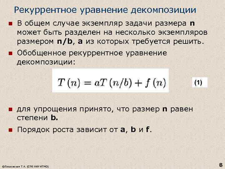 Recurrent Decomposition Equation n In general, an instance of a problem of size n can be divided into several instances of size n/b, from which it is required to solve. n Generalized recurrent decomposition equation: (1) n for simplicity, it is assumed that the size n is equal to the power b. n The order of growth depends on a, b and f. ©T. A. Pavlovskaya (St. Petersburg National Research University ITMO) 8
 Basic decomposition theorem (1) n You can specify the efficiency class of the algorithm without solving the recurrence equation itself. n This approach allows you to establish the order of growth of the solution without determining unknown factors. ©Pavlovskaya T. A. (St. Petersburg National Research University ITMO) 9
 Merge Sort Sorts a given array by splitting it into two halves, recursively sorting each half, and merging the two sorted halves into one sorted array: Mergesort (A) if n>1 First half A -> into array B Second half A -> into array C Mergesort(B) Mergesort(C) Merge(B, C, A) // merge © Pavlovskaya T. A. (SPb NRU ITMO) 10
Src="http://present5.com/presentation/54441564_438337950/image-11.jpg" alt="Mergesort (A) if n>1 First half of A -> to array B Second half of A"> Mergesort (A) if n>1 Первая половина А -> в массив В Вторая половина А > в массив С Mergesort(B) Mergesort(C) Меrgе(В, С, А) ©Павловская Т. А. (СПб НИУ ИТМО) 11!}
 Merging arrays n Two array indices after initialization point to the first elements of the merged arrays. n The elements are compared and the smaller one is added to new array. n The index of the smaller element is incremented (it points to the element immediately following the one just copied). This operation is repeated until one of the merged arrays is exhausted. The remaining elements of the second array are added to the end of the new array. ©Pavlovskaya T. A. (St. Petersburg National Research University ITMO) 12
 Merge Sort Analysis n Let the file length be a power of 2. n Number of key comparisons: C(n) = 2*C(n/2) + Cmerge (n) n > 1, C(1)=0 n Cmerge (n) = n-1 in the worst case (number of key comparisons during merging) n In the worst case Cw: d=1 a=2 b=2 Cw(n) = 2*Cw (n/2) +n-1 Cw (n ) (n log n) – according to basic. theorem ©Pavlovskaya T. A. (SPb NRU ITMO) (1) 13
 n The number of key comparisons performed by merge sort is, in the worst case, very close to the theoretical minimum number of comparisons for any comparison-based sort algorithm. n The main disadvantage of merge sort is the need for additional memory, the amount of which is linearly proportional to the size of the input data. ©T. A. Pavlovskaya (St. Petersburg National Research University ITMO) 14
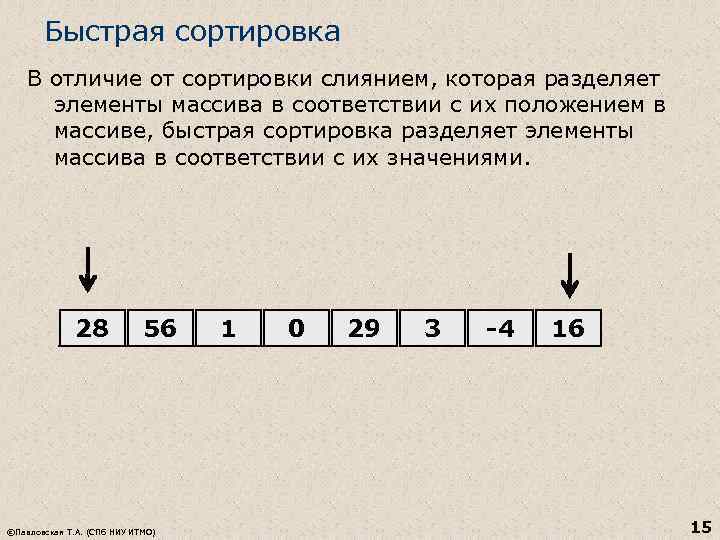 Quick Sort Unlike merge sort, which separates array elements according to their position in the array, quick sort separates array elements according to their values. 28 56 ©Pavlovskaya T. A. (St. Petersburg National Research University ITMO) 1 0 29 3 -4 16 15
 Description of the algorithm n Select a reference element n Perform a permutation of elements to obtain a partition when all elements up to some position s do not exceed element A [s], and elements after position s are not less than it. n Obviously, after partitioning, A [s] is in the final position, and we can sort the two subarrays of elements before and after A [s] independently (by the same or a different method) © T. A. Pavlovskaya (SPb NRU ITMO) 16
 Procedure for permuting elements n Effective method, based on two passes of the subarray - left to right and right to left. At each pass, the elements are compared with the reference. n Pass from left to right (i) skips elements smaller than the reference and stops at the first element not smaller than the reference. n The right to left pass (j) skips elements larger than the reference and stops at the first element not larger than the reference. n If the scanning indices do not intersect, we swap the found elements and continue passes. n If the indices intersect, exchange the support element with Aj © T. A. Pavlovskaya (St. Petersburg National Research University ITMO) 17
 Efficiency of quick sort n Best case: all partitions end up in the middle of the corresponding subarrays n In the worst case, all partitions turn out to be such that one of the subarrays is empty, and the size of the second is 1 less than the size of the partitioned array (quadratic dependence). n In the average case, we assume that the partition can be performed in each position with the same probability: Cavg 2 n ln n 1, 38 n log 2 n © T. A. Pavlovskaya (SPb NRU ITMO) 18
 Improvements to the algorithm n improved methods for selecting a reference element n switching to simpler sorting for small subarrays n removing recursion All together these improvements can reduce the running time of the algorithm by 20 -25% (R. Sedgwick) © T. A. Pavlovskaya (SPb NRU ITMO) 19
 Traversing a Binary Tree This is another example of using the decomposition method. n In preorder traversal, the root of the tree is first visited, and then the left and right subtrees. n In a symmetric traversal, the root is visited after the left subtree, but before visiting the right one. n When bypassing reverse order the root is visited after the left and right subtrees. ©Pavlovskaya T. A. (St. Petersburg National Research University ITMO) 20
 Traversing a tree procedure print_tree(tree); begin print_tree(left_subtree) visit the root print_tree(right_subtree) end; 1 6 8 10 20 ©Pavlovskaya T. A. (St. Petersburg State University ITMO) 21 25 30 21

 The problem size reduction method is based on using the connection between the solution of a given problem instance and the solution of a smaller instance of the same problem. Once such a relationship is established, it can be used either top-down (recursively) or bottom-up (non-recursive). (example - raising a number to a power) There are three main options for the method of reducing size: n reducing by a constant amount (usually by 1); n decrease by a constant factor (usually 2 times); n variable size reduction. ©Pavlovskaya T. A. (St. Petersburg National Research University ITMO) 23
 Insertion Sort Let's assume that the problem of sorting an array of dimension n-1 has been solved. Then all that remains is to insert An at the right place: n Looking through the array from left to right n Looking through the array from right to left n Using a binary search for the insertion location n Although insertion sort is based on a recursive approach, it is more efficient to implement it bottom-up (iterative). ©Pavlovskaya T. A. (St. Petersburg National Research University ITMO) 24
 Pseudocode implementation for i = 1 to n - 1 do v = 0 and A[j] > v do A
 Efficiency of insertion sort n Worst case: performs the same number of comparisons as selection sort n Best case (for an initially sorted array): compares only 1 time for each pass of the outer loop n Average case (random array): performs ~2 times fewer comparisons than in the case of a descending array. That. , the average case is 2 times better than the worst case. Coupled with its superior performance for nearly sorted arrays, this makes insertion sort stand out from other elementary (selection and bubble) algorithms. n A modification of the method is the insertion of several elements at a time, which are sorted before insertion. n An extension of insertion sort, Shell sort, provides an even better algorithm for sorting enough large files. ©Pavlovskaya T. A. (St. Petersburg National Research University ITMO) 26

 Generating Combinatorial Objects n The most important types of combinatorial objects are permutations, combinations, and subsets of a given set. n They typically arise in problems that require consideration of different choices. n In addition, there are the concepts of placement and partitioning. ©Pavlovskaya T. A. (St. Petersburg National Research University ITMO) 28
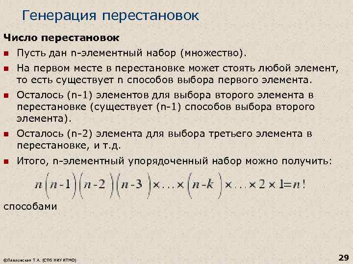 Generation of permutations Number of permutations n Let an n-element set (set) be given. n The first place in the permutation can be any element, that is, there are n ways to choose the first element. n There are (n-1) elements left to select the second element in the permutation (there are (n-1) ways to select the second element). n There are (n-2) elements left to select the third element in the permutation, etc. n Total, an n-element ordered set can be obtained: in ways © T. A. Pavlovskaya (SPb NRU ITMO) 29
 Applying the size reduction method to the problem of obtaining all permutations of n For simplicity, we assume that the set of elements to be permuted is the set of integers from 1 to n. n The task smaller by one is to generate all (n - 1)! permutations. n Assuming it has been solved, we can obtain a solution to the larger problem by inserting n into each of the n possible positions among the elements of each of the permutations of n - 1 elements. n All permutations obtained in this way will be different, and their total number: n(n- 1)! = n! n You can insert n into previously generated permutations from left to right or right to left. It is advantageous to start from right to left and change direction each time you move to a new permutation of the set (1, . . . , n - 1). ©Pavlovskaya T. A. (St. Petersburg National Research University ITMO) 30
 Example (ascending generation of permutations) n 12 21 n 123 132 312 321 231 213 © Pavlovskaya T. A. (SPb NRU ITMO) 31
 Johnson-Trotter algorithm The concept of a mobile element is introduced. Each element is associated with an arrow; an element is considered mobile if the arrow points to a smaller neighboring element. n Initialize the first permutation with the value 1 2. . . n (all arrows to the left) n while there is a mobile number k do n Find the largest mobile number k Swap k and the neighboring number pointed to by the arrow k n n Change the direction of the arrows for all numbers greater than k © Pavlovskaya T. A. (St. Petersburg National Research University ITMO) 32
 Lexicographical order n Let there be the first permutation (for example, 1234). n To find each next one: 1. Scan the current permutation from right to left in search of the first pair of neighboring elements such that a[i]
 An example to understand the algorithm 1234 1243 1324 1342 1423 1432 2134 2143 2314 2341 2413 2431 3124 3142 3214 3241 3412 3421 4123 4132 4213 4231 4312 43 21 ©Pavlovskaya T. A. (St. Petersburg National Research University ITMO) 34
 The number of all permutations of n elements P(n) = n! ©Pavlovskaya T. A. (St. Petersburg National Research University ITMO) 35
 Subsets n A set A is a subset of a set B if any element belonging to A also belongs to B: A B or A B n Any set is its own subset. The empty set is a subset of any set. n The set of all subsets is denoted by 2 A (it is also called power set, power set, degree of set, Boolean, exponential set). n The number of subsets of a finite set consisting of n elements is equal to 2 n (for the proof, see Wikipedia) © Pavlovskaya T. A. (SPb NRU ITMO) 36
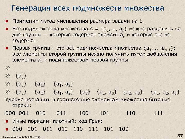 Generation of all subsets n Let us apply the method of reducing the size of the problem by 1. n All subsets A = (a 1, . . . , an) can be divided into two groups - those that contain the element an and those that do not contain it. n The first group is all subsets (a 1, . . . , an-1); all elements of the second group can be obtained by adding the element an to the subsets of the first group. (a 1) (a 2) (a 1, a 2) (a 3) (a 1, a 3) (a 2, a 3) (a 1, a 2, a 3) It is convenient to assign bit elements to the elements of the set lines: 000 001 010 011 100 101 110 111 n Other orders: dense; Gray code: n 000 001 010 111 100 ©T. A. Pavlovskaya (St. Petersburg National Research University ITMO) 37
 Generation of Gray codes n A Gray code for n bits can be recursively constructed from a code for n–1 bits by: n writing the codes in reverse order n concatenating the original and inverted lists n appending 0 to the beginning of each code in the original list and 1 to the beginning of the codes in an inverted list. Example: n Codes for n = 2 bits: 00, 01, 10 n Inverted list of codes: 10, 11, 00 n Combined list: 00, 01, 10, 11, 00 n Zeros added to the initial list: 000, 001, 010 , 11, 00 n Units added to the inverted list: 000, 001, 010, 111, 100 © Pavlovskaya T. A. (SPb NRU ITMO) 38
 K-element subsets n The number of k-element subsets n (0 k n) is called the number of combinations (binomial coefficient): n The direct solution is ineffective due to the rapid growth of the factorial. n As a rule, the generation of k-element subsets is carried out in lexicographic order (for any two subsets, the first to be generated is the one whose element indices can be used to form a smaller k-digit number in the n-ary number system). n Method: n the first element of a subset of cardinality k can be any of the elements, starting from the first and ending with the (n-k+1)th. n After the index of the first element of the subset is fixed, it remains to select k-1 elements from elements with indices greater than the first. n Further, similarly, reducing the problem to a smaller dimension until lowest level recursion will not be selected last element, after which the selected subset can be printed or processed. ©Pavlovskaya T. A. (St. Petersburg National Research University ITMO) 39
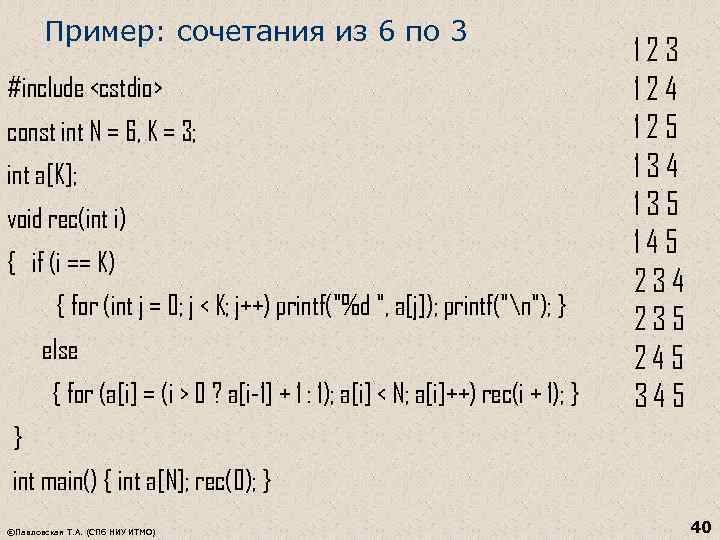 Example: combinations of 6 to 3 #include const int N = 6, K = 3; int a[K]; void rec(int i) ( if (i == K) ( for (int j = 0; j 0 ? a + 1: 1); a[i]
 Properties of combinations n Each n-element subset of a given element set corresponds to one and only one n-k-element subset of the same set: n © Pavlovskaya T. A. (SPb NRU ITMO) 41


 Placements n An arrangement of n elements by m is a sequence consisting of m different elements of some n-element set (combinations that are made up of given n elements by m elements and differ either in the elements themselves or in the order of the elements). Differences in the definitions of combinations and placements: n Combination – a subset containing m elements out of n (the order of the elements is not important). n An arrangement is a sequence containing m elements out of n (the order of the elements is important). When forming a sequence, the order of the elements is important, but when forming a subset, the order is not important. ©Pavlovskaya T. A. (St. Petersburg State University ITMO) 44
 Number of placements n Number of placements from n to m: Example 1: How many two-digit numbers are there in which the tens digit and the units digit are different and odd? Basic set: (1, 3, 5, 7, 9) – odd numbers, n=5 n Connection – two-digit number m=2, the order is important, which means this is a placement “of five by two”. n Permutations can be considered a special case of placements with m=n Example 2: In how many ways can a flag consisting of three horizontal stripes different colors if there is material in five colors? ©T. A. Pavlovskaya (St. Petersburg National Research University ITMO) 45
 Placements with repetitions n Placements with repetitions from n elements of the set E = (a 1, a 2, . . . , an) by k - any finite sequence consisting of k elements of a given set E. n Two placements with repetitions are considered different if at least in one place they have different elements of the set E. n The number of different placements with repetitions from n to k is equal to nk. ©Pavlovskaya T. A. (St. Petersburg National Research University ITMO) 46
 Partitioning of sets n Partitioning a set is its representation as a union of an arbitrary number of pairwise disjoint subsets. n The number of unordered partitions of an n-element set into k parts - the Stirling number of the 2nd kind: n The number of ordered partitions of an n-element set into m parts of a fixed size - a multinomial coefficient: n The number of all unordered partitions of an n-element set is given by the Bell number: © Pavlovskaya T. A. (SPb NRU ITMO) 47
 Reduction method by a constant factor n Example: binary search n Such algorithms are logarithmic and, being very fast, are quite rare. Method of reduction by a variable factor n Examples: search and insertion into a binary search tree, interpolation search: © Pavlovskaya T. A. (St. Petersburg State University ITMO) 48
 Performance Analysis n Interpolation search requires on average less than log 2 n+1 key comparisons when searching a list of n random values. n This function grows so slowly that for all real practical values of n it can be considered a constant. n However, in the worst case, the interpolation search degenerates into a linear search, which is considered as the worst possible search. n Interpolation search is best used for large files and for applications in which comparing or accessing data is an expensive operation. ©Pavlovskaya T. A. (St. Petersburg National Research University ITMO) 49
 Transformation method n Consists in the fact that an instance of a problem is transformed into another, for one reason or another easier to solve. n There are three main variants of this method: ©T. A. Pavlovskaya (St. Petersburg National Research University ITMO) 50
 Example 1: Checking the Uniqueness of Array Elements n A brute-force algorithm compares all elements pairwise until two identical ones are found or until all possible pairs have been reviewed. In the worst case, the efficiency is quadratic. n You can approach the problem in another way - first sort the array and then compare only consecutive elements. n The running time of the algorithm is the sum of the sorting time and the time for checking neighboring elements. n If you use a good sorting algorithm, the entire algorithm for checking the uniqueness of array elements will also have an efficiency of O (n log n) © T. A. Pavlovskaya (SPb NRU ITMO) 51