Practical work on olap technology in excel. Finance in Excel. Some information about OLAP cubes and Power Pivot data models

1 task (general) (2 points).

Using a spreadsheet, process data using statistical functions.
1. Information is given about the students of the class (10 people), including grades for one month in mathematics. Count the number of fives, fours, twos and threes, find the average score of each student and the average score of the entire group. Create a chart illustrating the percentage of grades in a group.

2.1 task (2 points).

Four friends travel by three modes of transport: train, plane and ship. Nikolai sailed 150 km by boat, traveled 140 km by train and flew 1100 km by plane. Vasily sailed 200 km by boat, traveled 220 km by train and flew 1160 km by plane. Anatoly flew 1200 km by plane, traveled 110 km by train and sailed 125 km by boat. Maria traveled 130 km by train, flew 1500 km by plane and sailed 160 km by boat.
Build a spreadsheet based on the above data.

Add a column to the table that will display the total number of kilometers that each of the guys traveled.

Calculate the total number of kilometers that the children traveled by train, flew by plane and sailed by boat (on each type of transport separately).

Calculate the total number of kilometers of all friends.

Determine the maximum and minimum number of kilometers traveled by friends using all types of transport.

Determine the average number of kilometers for all types of transport.

2.2 task (2 points).

Create a table “Lakes of Europe” using the following data on area (sq. km) and greatest depth (m): Ladoga 17,700 and 225; Onega 9510 and 110; Caspian Sea 371,000 and 995; Wenern 5550 and 100; Chudskoye with Pskovsky 3560 and 14; Balaton 591 and 11; Geneva 581 and 310; Wettern 1900 and 119; Constance 538 and 252; Mälaren 1140 and 64. Determine the largest and smallest lake in area, the deepest and shallowest lake.

2.3 task (2 points).

Create a table “Rivers of Europe” using the following length (km) and basin area (thousand sq. km): Volga 3688 and 1350; Danube 2850 and 817; Rhine 1330 and 224; Elbe 1150 and 148; Vistula 1090 and 198; Loire 1020 and 120; Ural 2530 and 220; Don 1870 and 422; Sena 780 and 79; Thames 340 and 15. Determine the longest and shortest river, calculate the total area of ​​river basins, the average length of rivers in the European part of Russia.

Task 3 (2 points).

The bank records the timeliness of payments of loans issued to several organizations. The loan amount and the amount already paid by the organization are known. Penalties are established for debtors: if the company has repaid the loan by more than 70 percent, the fine will be 10 percent of the debt amount, otherwise the fine will be 15 percent. Calculate the fine for each organization, the average fine, the total amount of money that the bank is going to receive additionally. Determine the average fine of budgetary organizations.

Find material for any lesson,

Amazing - close...

In the course of my work, I often needed to make complex reports, I was always trying to find something common in them in order to compile them more simply and universally, I even wrote and published an article on this subject, “Osipov’s Tree.” However, my article was criticized and they said that all the problems that I raised had long been solved in MOLAP.RU v.2.4 (www.molap.rgtu.ru) and they recommended looking at the pivot tables in EXCEL.
It turned out to be so simple that, having applied my ingenious little hands to it, I came up with a very simple scheme for downloading data from 1C7 or any other database (hereinafter, 1C means any database) and analysis in OLAP.
I think many OLAP upload schemes are too complicated, I choose simplicity.

Characteristics :

1. Only EXCEL 2000 is required for work.
2. The user can design reports himself without programming.
3. Uploading from 1C7 in a simple text file format.
4. For accounting entries, there is already a universal processing for unloading that works in any configuration. Sample processing is available for downloading other data.
5. You can design report forms in advance and then apply them to different data without re-designing them.
6. Quite good performance. At the first long stage, the data is first imported into EXCEL from a text file and an OLAP cube is built, and then pretty quickly any report can be built on the basis of this cube. For example, data on product sales for a store for 3 months with an assortment of 6000 products is loaded into EXCEL in 8 minutes on Cel600-128M, the rating by product and group (OLAP report) is recalculated in 1 minute.
7. Data is downloaded from 1C7 in full for the specified period (all movements, across all warehouses, companies, accounts). When importing into EXCEL, it is possible to use filters that load only the necessary data for analysis (for example, from all movements, only sales).
8. Currently, methods have been developed for analyzing movements or residues, but not movements and residues together, although this is possible in principle.

What is OLAP : (www.molap.rgtu.ru)

Let's say you have a retail chain. Let the data on trading operations be uploaded to a text file or table like this:

Date - date of operation
Month - month of operation
Week - week of operation
Type - purchase, sale, return, write-off
Counterparty - an external organization participating in a transaction
Author - the person who issued the invoice

In 1C, for example, one row of this table will correspond to one line of the invoice; some fields (Counterparty, Date) are taken from the invoice header.

Data for analysis is usually uploaded into an OLAP system for a certain period of time, from which, in principle, another period can be selected using loading filters.

This table is the source for OLAP analysis.

The user himself determines which of the table fields will be Dimensions, which Data and which Filters to apply. The system itself builds a report in a visual tabular form. Dimensions can be placed in the row or column headings of a report table.
As you can see, from one simple table you can get a lot of data in the form of various reports.

How to use it yourself :

Unpack the data from the distribution exactly into the c:\fixin directory (for a trading system it is possible in c:\reports). Read the readme.txt and follow all the instructions in it.

First you must write a processing that uploads data from 1C to a text file (table). You need to determine the composition of the fields that will be unloaded.
For example, ready-made universal processing, which works in any configuration and downloads transactions for a period for OLAP analysis, downloads the following fields for analysis:

Date|Day of the Week|Week|Year|Quarter|Month|Document|Company|Debit|DtNomenclature
|DtGroupNomenclature|DtSectionNomenclature|Credit|Amount|ValAmount|Quantity
|Currency|DtCounterparties|DtGroupCounterparties|KtCounterparties|KtGroupCounterparties|
CTMiscellaneousObjects

Where under the prefixes Dt(Kt) there are subaccounts of Debit (Credit), Group is the group of this subaccount (if any), Section is the group of the group, Class is the group of the section.

For a trading system, the fields can be as follows:

Direction|Type of Movement|For Cash|Product|Quantity|Price|Amount|Date|Company
|Warehouse|Currency|Document|Day of the Week|Week|Year|Quarter|Month|Author
|Product Category|Movement Category|Counterparty Category|Product Group
|ValAmount|Cost|Counterparty

To analyze the data, the tables "Movement Analysis.xls" ("Accounting Analysis.xls") are used. When opening them, do not disable macros, otherwise you will not be able to update the reports (they are run by VBA macros). These files take their source data from the files C:\fixin\motions.txt (C:\fixin\buh.txt), otherwise they are the same. Therefore, you may have to copy your data to one of these files.
To load your data into EXCEL, select or write your filter and click the “Generate” button on the “Conditions” sheet.
Report sheets begin with the prefix "Report". Go to the report sheet, click "Refresh" and the report data will change according to the last loaded data.
If you are not satisfied with standard reports, there is a ReportTemplate sheet. Copy it to a new sheet and customize the report type by working with a pivot table on this sheet (about working with pivot tables - in any EXCEL 2000 book). I recommend setting up reports on a small set of data, and then running them on a large array, because... There is no way to disable redrawing of tables every time the report layout changes.

Technical Notes :

When uploading data from 1C, the user selects the folder where to upload the file. I did this because it is likely that there will be multiple files being uploaded (leftovers and movements) in the near future. Then, by clicking the “Submit” button in Explorer --> “To OLAP analysis in EXCEL 2000,” the data is copied from the selected folder to the C:\fixin folder. (for this command to appear in the list of the “Send” command, you need to copy the file “For OLAP analysis in EXCEL 2000.bat” to the C:\Windows\SendTo directory) Therefore, upload the data immediately by naming the files motions.txt or buh.txt.

Text file format:
The first line of the text file is the column headers separated by "|", the remaining lines contain the values ​​of these columns separated by "|".

To import text files into Excel, Microsoft Query (a component of EXCEL) is used; for it to work, you must have a shema.ini file containing the following information in the import directory (C:\fixin):

ColNameHeader=True
Format=Delimited(|)
MaxScanRows=3
CharacterSet=ANSI
ColNameHeader=True
Format=Delimited(|)
MaxScanRows=3
CharacterSet=ANSI

Explanation: motions.txt and buh.txt are the name of the section, corresponds to the name of the imported file, describes how to import a text file into Excel. The remaining parameters mean that the first line contains the names of the columns, the column separator is "|", the character set is Windows ANSI (for DOS - OEM).
The field type is determined automatically based on the data contained in the column (date, number, string).
The list of fields does not need to be described anywhere - EXCEL and OLAP will themselves determine which fields are contained in the file by the headings in the first line.

Attention, check your regional settings "Control Panel" --> "Regional Settings". In my processing, numbers are uploaded with a comma delimiter, and dates are in the format "DD.MM.YYYY".

When you click the "Generate" button, the data is loaded into the pivot table on the "Base" sheet, and all reports on the "Report" sheets take data from this pivot table.

I understand that fans of MS SQL Server and powerful databases will begin to grumble that everything is too simplified, that my processing will be exhausted by a year-long sample, but first of all I want to give the benefits of OLAP analysis to medium-sized organizations. I would position this product as an annual analysis tool for wholesale companies, quarterly analysis for retailers, and operational analysis for any organization.

I had to tinker with VBA so that the data could be taken from a file with any list of fields and I could prepare report forms in advance.

Description of work in EXCEL (for users):

Instructions for using reports:
1. Send the downloaded data for analysis (check with the administrator). To do this, right-click on the folder into which you downloaded data from 1C and select the “Send” command, then “To OLAP analysis in EXCEL 2000”.
2. Open the file "Motion Analysis.xls"
3. Select Filter Value; the filters you need can be added on the “Values” tab.
4. Click the "Generate" button, and the downloaded data will be loaded into EXCEL.
5. After loading the data into EXCEL, you can view various reports. To do this, just click the "Refresh" button in the selected report. Report sheets begin with Report.
Attention! After you change the filter value, you need to click the “Generate” button again so that the data in EXCEL is reloaded from the upload file in accordance with the filters.

Processing from the demo example:

Processing motionsbuh2011.ert - the latest version of uploading transactions from Accounting 7.7 for analysis in Excel. It has a checkbox “Attach to file”, which allows you to upload data in parts by period, appending it to the same file, rather than uploading it to the same file again:

Processing motionswork.ert uploads sales data for analysis in Excel.

Examples of reports:

Wiring chess:

Operator workload by types of invoices:

P.S. :

It is clear that a similar scheme can be used to organize the downloading of data from 1C8.
In 2011, a user contacted me who needed to improve this processing in 1C7 so that it would upload large amounts of data, I found an outsourcer and did the work. So the development is quite relevant.

The processing of motionsbuh2011.ert has been improved to cope with unloading large amounts of data.

In a standard pivot table, the source data is stored on your local hard drive. This way, you can always manage and reorganize them, even without access to the network. But this in no way applies to OLAP pivot tables. In OLAP pivot tables, the cache is never stored on the local hard drive. Therefore, immediately after disconnecting from the local network, your pivot table will no longer work. You will not be able to move a single field in it.

If you still need to analyze OLAP data after going offline, create an offline data cube. An offline data cube is a separate file that is a pivot table cache and stores OLAP data that is viewed after disconnecting from the local network. OLAP data copied into a pivot table can be printed; this is described in detail on the website http://everest.ua.

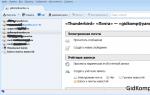
To create a standalone data cube, first create an OLAP pivot table. Place the cursor within the pivot table and click on the OLAP Tools button on the Tools contextual tab, which is part of the PivotTable Tools contextual tab group. Select the Offline OLAP command (Fig. 9.8).

Rice. 9.8. Create an offline data cube

The Offline OLAP Data Cube Settings dialog box appears on the screen. Click on the Create Offline Data File button. You have launched the Create Data Cube File Wizard. Click the Next button to continue the procedure.

First you need to specify the dimensions and levels that will be included in the data cube. In the dialog box, you must select the data that will be imported from the OLAP database. The idea is to specify only those dimensions that will be needed after the computer is disconnected from the local network. The more dimensions you specify, the larger the autonomous data cube will be.

Click the Next button to move to the next wizard dialog box. This gives you the ability to specify members or data elements that will not be included in the cube. In particular, you won't need the Internet Sales-Extended Amount measure, so its checkbox will be cleared in the list. A cleared check box indicates that the specified item will not be imported and take up unnecessary space on your local hard drive.

In the last step, specify the location and name of the data cube. In our case, the cube file will be named MyOfflineCube.cub and will be located in the Work folder.

Data cube files have the extension .cub

After some time, Excel will save the offline data cube in the specified folder. To test it, double-click on the file, which will automatically generate an Excel workbook that contains a pivot table associated with the selected data cube. Once created, you can distribute the offline data cube to all interested users who are working in offline LAN mode.

Once connected to your local network, you can open the offline data cube file and update it and the associated data table. The main principle states that the offline data cube is used only to work when the local network is disconnected, but it is required to be updated after the connection is restored. Attempting to update an offline data cube after a connection failure will result in a failure.

Working with offline cube files

An offline cube file (.cub) stores data in the form of an OLAP (Online Analytical Processing) cube. This data may represent part of the OLAP database on the OLAP server or may be created independently of the OLAP database. Use an offline cube file to continue working with PivotTable and PivotChart reports when the server is unavailable or when you are offline.

Safety Note: Be careful when using or distributing an offline cube file that contains sensitive or personal data. It is recommended that you save the data in a workbook instead of a cube file so that you can control access to the data using rights management. additional information can be found in Manage information rights in Office.

When working with a PivotTable or PivotChart report that is based on OLAP server source data, you can use the Offline Cube Wizard to copy the source data to separate file offline cube on a computer. To create these offline files, your OLAP data provider must support this capability, such as MSOLAP from Microsoft Services SQL Server Analysis Services installed on the computer.

Note: Create and use offline cube files from services Microsoft SQL Server Analysis Services is subject to terms and licensing Microsoft installations SQL Server. Review the applicable SQL Server version licensing information.

Working with the Offline Cube Wizard

To create an offline cube file, you can select a subset of data in an OLAP database using the Offline Cube Wizard and then save the subset. The report does not need to include all the fields included in the file, nor does it need to select any of them and the data fields available in the OLAP database. To keep the file at a minimum, you can only include the data you want to appear in the report. You can omit all dimensions and for most types of dimensions you can also exclude lower level information and items top level, which do not need to be displayed. For all elements that you include, the property fields available in the database for those elements are also saved in an offline file.

Taking data offline and connecting it back

To do this, you first need to create a PivotTable or PivotChart report that is based on the server database, and then create an offline cube file from the report. You can then switch the report between the server database and the offline file at any time. For example, if you use a laptop for home work and video trips, then reconnect the computer to the network.

Below are the basic steps you need to follow to battery life with the data and then transfer the data back to the Internet.

Create or open a PivotTable or PivotChart report based on OLAP data that you want to access offline.

Create an offline cube file on your computer. In chapter Creating an offline cube file from an OLAP server database(lower in this article).

Disconnecting from the network and working with the offline cube file.

Connect to the network and reconnect the cube file offline. Check out the section Reconnecting the offline cube file to the OLAP server database(below in this article).

Update the offline cube file with new data and recreate the offline cube file. Check out the section updating and re-creating the offline cube file(lower in this article).

BLOG

Only quality posts

What are Excel Pivot Tables and OLAP Cubes

Watch the video for the article:

OLAP- this is English. online analytical processing, analytical technology for processing data in real time. In simple terms - a warehouse with multidimensional data (Cube), even simpler - just a database from which you can get data in Excel and analyze it using the Excel tool - Pivot Tables.

Pivot tables is a user interface for displaying multidimensional data. In other words, it is a special type of table that can be used to create almost any report.

To make it clear, let's compare a "Regular Table" with a "Pivot Table"

Regular table:

Summary table:

Main difference Pivot tables– this is the presence of a window “ List of Pivot Table Fields", from which you can select the required fields and get any table automatically!

How to use

Open an Excel file that is connected to an OLAP cube, for example "BIWEB":

Now, what does this mean and how to use it?

Drag and drop the required fields to get, for example, a table like this:

« Pluses» allow you to drill down into the report. In this example, “Brand” is detailed to “Abbreviated Names”, and “Quarter” to “Month”, i.e. So:

Analytical functions in Excel (cube functions)

Microsoft is constantly adding new capabilities to Excel in terms of data analysis and visualization. Working with information in Excel can be represented as relatively independent three layers:

• “correctly” organized source data
• mathematics (logic) of data processing
• data presentation

Rice. 1. Data analysis in Excel: a) source data, b) measure in Power Pivot, c) dashboard; To enlarge the image click on it right click mouse and select Open image in new tab

Download the note in Word or pdf format, examples in Excel format

Cube functions and pivot tables

The simplest and at the same time very powerful means of presenting data are pivot tables. They can be built on the basis of data contained in: a) an Excel sheet, b) an OLAP cube or c) a model Data Power Pivot. In the last two cases, in addition to the pivot table, you can use analytical functions (cube functions) to generate a report on an Excel sheet. Pivot tables are simpler. Cube functions are more complex, but provide more flexibility, especially in report design, which is why they are widely used in dashboards.

The following discussion applies to cube formulas and pivot tables based on the Power Pivot model and, in a few cases, based on OLAP cubes.

Easy way to get cube functions

When (if) you started learning VBA code, you learned that the easiest way to get to the code is to use macro recording. Then the code can be edited, loops, checks, etc. can be added. Similarly, the easiest way to obtain a set of cube functions is to transform the pivot table (Fig. 2). Stand on any cell of the pivot table, go to the tab Analysis, click on the button Facilities OLAP, and press Convert to formulas.

Rice. 2. Convert a PivotTable to a Cube Function Set

The numbers will be saved, and these will not be values, but formulas that extract data from the Power Pivot data model (Figure 3). You can format the resulting table. Including, you can delete and insert rows and columns inside the table. The slice remains and it affects the data in the table. When the source data is updated, the numbers in the table will also update.

Rice. 3. Table based on cube formulas

CUBEVALUE() function

This is perhaps the main function of cubes. She is equivalent to the area Values pivot table. CUBEVALUE retrieves data from a cube or Power Pivot model and displays it outside of a PivotTable. This means you are not limited by the PivotTable and can create reports with countless possibilities.

Writing a formula from scratch

You don't have to convert a pre-built PivotTable. You can write any cube formula from scratch. For example, the following formula is entered into cell C10 (Fig. 4):

Rice. 4. The CUBEVALUE() function in cell C10 returns bicycle sales for all years, as in the pivot table

A little trick. To make it easier to read cube formulas, it is advisable that only one argument be placed on each line. You can make the Excel window smaller. To do this, click on the icon Roll out the window, located in the upper right corner of the screen. And then adjust the window size horizontally. Alternative option– force the text of the formula to be moved to a new line. To do this, in the formula bar, place the cursor in the place where you want to make the transfer and press Alt+Enter.

Rice. 5. Minimize the window

Syntax of the CUBEVALUE() function

Excel help is completely accurate and completely useless for beginners:

CUBEVALUE(connection; [element_expression1]; [element_expression2]; ...)

Connection– required argument; a text string representing the name of the connection to the cube.

Element_expression– optional argument; a text string representing an MDX that returns an element or tuple in a cube. Additionally, "element_expression" can be a set defined using the CUBESET function. Use "element_expression" as a slice to determine the part of the cube for which you want to return an aggregated value. If no measure is specified in element_expression, the default measure for that cube will be used.

Before we go on to explain the syntax of the CUBEVALUE function, a few words about cubes, data models, and the mysterious motorcade.

Some information about OLAP cubes and Power Pivot data models

OLAP data cubes ( O n l ine A nalytical P rocessing - operational data analysis) were developed specifically for analytical processing and quick extraction of data from them. Imagine a three-dimensional space where time periods, cities and goods are plotted along the axes (Fig. 5a). The nodes of such a coordinate grid contain the values ​​of various measures: sales volume, profit, costs, number of units sold, etc. Now imagine that there are dozens, or even hundreds of dimensions... and there are also a lot of measures. This will be a multidimensional OLAP cube. Creating, configuring and maintaining OLAP cubes is the job of IT specialists.

Rice. 5a. 3D OLAP cube

Excel analytical formulas (cube formulas) extract axis names (for example, Time), names of elements on these axes (August, September), values ​​of measures at the intersection of coordinates. It is this structure that allows cube-based pivot tables and cube formulas to be so flexible and adapt to the needs of users. Pivot tables based on Excel sheets do not use measures, so they are not as flexible for data analysis purposes.

Power Pivot is a relatively new Microsoft feature. This is a built-in Excel and partly independent environment with a familiar interface. Power Pivot is much more powerful than standard pivot tables. At the same time, developing cubes in Power Pivot is relatively simple, and most importantly, it does not require the participation of an IT specialist. Microsoft is implementing its slogan: “Business analytics to the masses!” Although Power Pivot models are not 100% cubes, they can also be considered cubes (for more information, see Mark Moore's introductory course, Power Pivot, and Rob Colley's longer course, DAX Formulas for Power Pivot).

The main components of a cube are dimensions, hierarchies, levels, elements (or members; in English members) and measures (measures). Measurement – main characteristics of the analyzed data. For example, product category, time period, sales geography. A dimension is something we can place on one of the axes of a pivot table. Each dimension, in addition to unique values, includes an element that performs an aggregation of all elements of this dimension.

Measurements are based on hierarchy. For example, a product category can be divided into subcategories, then into models, and finally into product names (Fig. 5b). Hierarchy allows you to create summary data and analyze it at various levels of the structure. In our example, the hierarchy Category includes 4 Level.

Elements(individual members) are present at all levels. For example, at the Category level there are four elements: Accessories, Bikes, Clothing, Components. Other levels have their own elements.

Measures– these are calculated values, for example, sales volume. Measures in cubes are stored in their own dimension called (see Figure 9 below). Measures do not have hierarchies. Each measure calculates and stores a value for all dimensions and all elements, and is sliced ​​depending on which dimension elements we place on the axis. They also say what coordinates we will set, or what filter context we will set. For example, in Fig. 5a, in each small cube the same measure is calculated - Profit. And the value returned by the measure depends on the coordinates. On the right, Figure 5a shows that Profit (in three coordinates) in Moscow in October on apples = 63,000 rubles. A measure can also be interpreted as one of the dimensions. For example, in Fig. 5a instead of an axis Goods, place the axis Measures with elements Volume of sales, Profit, Units sold. Then each cell will be some value, for example, Moscow, September, sales volume.

Cortege– several elements of different dimensions that specify coordinates along the cube axes in which we calculate the measure. For example, in Fig. 5a Cortege= Moscow, October, apples. Also an acceptable tuple is Perm, apples. Another one – apples, August. Dimensions not included in the tuple are present in it implicitly, and are represented by the default member. Thus, a cell of a multidimensional space is always defined by a complete set of coordinates, even if some of them are omitted from the tuple. You cannot include two elements of the same dimension in a tuple, the syntax won’t allow it. For example, an invalid tuple Moscow and Perm, apples. To implement such a multidimensional expression, you will need a set of two tuples: Moscow and apples + Perm and apples.

Set of elements– several elements of one dimension. For example, apples and pears. Set of tuples– several tuples, each of which consists of the same dimensions in the same sequence. For example, a set of two tuples: Moscow, apples and Perm, bananas.

Auto-completion to help

Let's return to the syntax of the CUBEVALUE function. Let's use auto-completion. Start entering a formula in a cell:

Excel will suggest all available in Excel workbook connections:

Rice. 6. The connection to the Power Pivot data model is always called ThisWorkbookDataModel

Rice. 7. Connections to cubes

Let's continue entering the formula (in our case for the data model):

Autocomplete will suggest all available tables and measures in the data model:

Rice. 8. Available elements of the first level - table names and a set of measures (highlighted)

Select an icon Measures. Make a point:

CUBEVALUE(" ThisWorkbookDataModel " ; " .

Autocomplete will suggest all available measures:

Rice. 9. Available second-level elements in the measure set

Select a measure. Add quotation marks, a closing parenthesis, and press Enter.

CUBEVALUE(" ThisWorkbookDataModel " ; " . " )

Rice. 10. CUBE VALUE formula in an Excel cell

Similarly, you can add a third argument to the formula:

VBA in Excel Excel.PivotTable object and working with pivot tables and OLAP cubes in Excel

10.8 Working with pivot tables (PivotTable object)

Excel.PivotTable object, program work with pivot tables and OLAP cubes in Excel using VBA, PivotCache object, creating a pivot table layout

During the operation of most enterprises, so-called raw data about activities accumulate. For example, for a trading enterprise, data on sales of goods can be accumulated - for each purchase separately, for enterprises cellular communication- load statistics on base stations, etc. Very often, the management of an enterprise needs analytical information that is generated on the basis of raw information - for example, to calculate the contribution of each type of product to the income of the enterprise or the quality of service in the area of ​​​​a given station. It is very difficult to extract such information from raw information: you need to run very complex SQL queries that take a long time to execute and often interfere with the current work. Therefore, increasingly, raw data is now consolidated first into an archival data warehouse - the Data Warehouse, and then into OLAP cubes, which are very convenient for interactive analysis. The easiest way to think of OLAP cubes is as multidimensional tables, in which, instead of the standard two dimensions (columns and rows, as in regular tables), there can be a lot of dimensions. The term "sectional" is commonly used to describe measurements in a cube. For example, the marketing department may need information by time, by region, by product type, by sales channel, etc. Using cubes (as opposed to standard SQL queries), it is very easy to get answers to questions like “how many products of this type were sold in the fourth quarter of last year in the North-West region through regional distributors.

Of course, such cubes cannot be created in conventional databases. Working with OLAP cubes requires specialized software products. SQL Server comes with an OLAP database from Microsoft called Analysis Services. There are OLAP solutions from Oracle, IBM, Sybase, etc.

To work with such cubes, Excel has a built-in client. In Russian it is called Pivot table(on graphic screen it is available through the menu Data -> Pivot table), and in English - Pivot Table. Accordingly, the object that this client represents is called a PivotTable. It should be noted that it can work not only with OLAP cubes, but also with regular data in Excel tables or databases, but many opportunities are lost.

The PivotTable and PivotTable are software products from Panorama Software that were acquired by Microsoft and integrated into Excel. Therefore, working with the PivotTable object is somewhat different from working with others. Excel objects. Figuring out what needs to be done is often difficult. Therefore, it is recommended to actively use the macro recorder to receive hints. At the same time, when working with pivot tables, users often have to perform the same repetitive operations, so automation is necessary in many situations.

What does working with a pivot table look like programmatically?

The first thing we need to do is create a PivotCache object that will represent a set of records retrieved from the OLAP source. Very roughly, this PivotCache object can be compared to a QueryTable. You can only use one PivotCache object per PivotTable object. A PivotCache object is created using the Add() method of the PivotCaches collection:

Dim PC1 As PivotCache

Set PC1 = ActiveWorkbook.PivotCaches.Add(xlExternal)

PivotCaches is a standard collection, and among the methods that deserve detailed consideration, only the Add() method can be named in it. This method takes two parameters:

• SourceType- required, defines the type of data source for the pivot table. You can specify the creation of a PivotTable based on a range in Excel, data from a database, an external data source, another PivotTable, etc. In practice, it usually makes sense to use OLAP only when there is a lot of data - accordingly, you need specialized external storage (for example, Microsoft Analysis Services). In this situation, the xlExternal value is selected.
• SourceData- required in all cases, except when the value of the first parameter is xlExternal. In fact, it defines the data range on the basis of which the PivotTable will be created. Typically takes a Range object.

The next task is to configure the PivotCache object settings. As already mentioned, this object is very similar to QueryTable, and its set of properties and methods is very similar. Some of the most important properties and methods:

• ADOConnection- the ability to return an ADO Connection object that is automatically created to connect to an external data source. Is used for additional settings connection properties.
• Connection- works exactly the same as the QueryTable object property of the same name. Can accept a connection string, a ready-made Recordset object, text file,Web query. Microsoft file Query. Most often, when working with OLAP, the connection string is written directly (since getting a Recordset object, for example, to change data, does not make much sense - OLAP data sources are almost always read-only). For example, setting this property to connect to the Foodmart database (Analysis Services sample database) on the LONDON server might look like this:

PC1.Connection = "OLEDB;Provider=MSOLAP.2;Data Source=LONDON1;Initial Catalog = FoodMart 2000"

• properties CommandType And CommandText they also describe the type of command that is sent to the database server and the text of the command itself. For example, to access the Sales cube and get it entirely into the cache on the client, you can use code like

• property LocalConnection allows you to connect to a local cube (*.cub file) created using Excel. Of course, it is not recommended to use such files for working with “production” volumes of data - only for the purpose of creating layouts, etc.
• property MemoryUsed returns quantity random access memory, used by PivotCache. If a PivotTable based on this PivotCache has not yet been created and opened, it returns 0. Can be used for checks if your application will run on weak clients.
• property OLAP returns True if PivotCache is connected to the OLAP server.
• OptimizeCache- ability to optimize the cache structure. The initial data download will take longer, but then the speed may increase. Doesn't work for OLE DB sources.

The remaining properties of the PivotCache object are the same as those of the QueryTable object, and therefore will not be discussed here.

The main method of the PivotCache object is the CreatePivotTable() method. Using this method, the next stage is performed - creating a pivot table (PivotTable object). This method takes four parameters:

• TableDestination- the only required parameter. Accepts a Range object in the upper left corner of which the pivot table will be placed.
• TableName- name of the pivot table. If not specified, the view name “PivotTable1” will be automatically generated.
• ReadData- if set to True, then the entire contents of the cube will be automatically placed in the cache. You need to be very careful with this parameter, since using it incorrectly can dramatically increase the load on the client.
• DefaultVersion- this property is usually not specified. Allows you to determine the version of the pivot table being created. By default, the most recent version is used.

Creating a pivot table in the first cell of the first worksheet might look like this:

PC1.CreatePivotTable Range("A1")

We have created a pivot table, but immediately after creation it is empty. It provides four areas in which you can place fields from the source (on the graphical screen all this can be configured either using the window List of Pivot Table Fields- it opens automatically or using a button Layout on the last screen of the PivotTable Wizard):

• column area- it contains those dimensions (“section” in which the data will be analyzed) whose members are smaller;
• line area- those dimensions which have more members;
• page area- those measurements for which you only need to filter (for example, show data only for such and such a region or only for such and such a year);
• data area- in fact, the central part of the table. Those numerical data (for example, the amount of sales) that we analyze.

Relying on the user to place elements correctly in all four areas is difficult. Additionally, it may take certain time. Therefore, it is often necessary to arrange data in a pivot table programmatically. This operation is performed using the CubeField object. The main property of this object is Orientation, it determines where this or that field will be located. For example, let's place the Customers dimension in the columns area:

PT1.CubeFields("").Orientation = xlColumnField

Then - the Time measurement into the line area:

PT1.CubeFields("").Orientation = xlRowField

Then - the Product dimension to the page area:

PT1.CubeFields("").Orientation = xlPageField

And finally, the indicator (numeric data for analysis) Unit Sales:

PT1.CubeFields(“.”).Orientation = xlDataField

Problems of analytics, OLAP, and data warehouses are of increasing interest to Russian IT specialists. To date, many good materials on this topic, including introductory ones, have been published in our computer press and on the Internet. We bring to your attention an article in which we deliberately try to explain OLAP “at a glance”, using a specific example. Practice shows that such an explanation is necessary for some IT specialists and especially end users.

So, OLAP *1, to a first approximation, “at a glance”, can be defined as a special way of analyzing data and obtaining reports. Its essence is to provide the user with a multidimensional table that automatically summarizes data in various sections and allows interactive management of calculations and report form. This article will talk about the technology and basic operations of OLAP using the example of analyzing invoices of an enterprise engaged in the wholesale trade of food products.

*1. OLAP - On-Line Analytical Processing, operational data analysis.

The OLAP system of the simplest and most inexpensive class will be considered as a tool - OLAP client *1. For example, we selected the simplest product among OLAP clients - “Contour Standard” from Intersoft Lab. (For clarity, later in the article, generally accepted OLAP terms will be indicated in bold and accompanied by their English equivalents.)

*1. More details about the classification of OLAP systems are described in the article “OLAP, made in Russia” in PC Week/RE, No. 3/2001.

So, let's get started with the system. First you need to describe the data source - the path to the table and its fields. This is the task of the user who knows the physical implementation of the database. For end users, it translates the name of the table and its fields into domain terms. Behind the “data source” is a local table, SQL server table or view, or stored procedure.

Most likely, in a particular database, invoices are stored not in one, but in several tables. In addition, some fields or records may not be used for analysis. Therefore, a Selection (result set or query) is then created, in which the following are configured: the algorithm for combining tables by key fields, filtering conditions and the set of returned fields. Let’s call our selection “Invoices” and place all the fields of the “Invoices” data source into it. Thus, the IT specialist, by creating a semantic layer, hides the physical implementation of the database from the end user.

Then the OLAP report is configured. This can be done by a subject matter expert. First, the fields of a flat data sample are divided into two groups - facts (facts or measures) and dimensions (dimensions). Facts are numbers, and measurements are “sections” in which the facts will be summarized. In our example, the dimensions will be: “Region”, “City”, “Customer”, “Product”, “Date”, and there will be one fact - the “Amount” field of the invoice. For a fact, you need to select one or more aggregation algorithms. OLAP is capable of not only summarizing results, but also performing more complex calculations, including statistical analysis. Selecting multiple aggregation algorithms will create virtual, calculated facts. In the example, one aggregation algorithm is selected - “Sum”.

A special property of OLAP systems is the generation of measurements and data for older time periods from a date and the automatic calculation of totals for these periods. Let’s select the periods “Year”, “Quarter” and “Month”, while data for each day will not be in the report, but the generated dimensions “Year”, “Quarter” and “Month” will appear. Let's name the report “Sales Analysis” and save it. The work on creating the interface for the analytical application is completed.

Now, when running this interface daily or monthly, the user will see a table and graph that summarizes invoices by item, customer, and period.

In order for data manipulation to be intuitive, the tools for managing a dynamic table are the elements of the table itself - its columns and rows. The user can move them, delete them, filter them, and perform other OLAP operations. In this case, the table automatically calculates new intermediate and final totals.

For example, by dragging (“move” operation) the “Product” column to the first place, we will receive a comparison report - “Comparison of product sales volumes for the year.” To aggregate data for a year, just drag the “Quarter” and “Month” columns to the top of the table - the “inactive dimensions area”. The “Quarter” and “Month” dimensions transferred to this area will be closed (“close dimension” operation), i.e. excluded from the report; in this case, the facts are summarized for the year. Despite the fact that the dimensions are closed, you can set specific years, quarters and months for them to filter the data (“filter” operation).

For greater clarity, let's change the type of graph illustrating the OLAP table and its location on the screen.

Digging deeper into the data (“drill down” operation) allows us to obtain more detailed information about the sales of the product we are interested in. By clicking on the “+” sign next to the “Coffee” product, we will see its sales volumes by region. Having expanded the “Ural” region, we will get sales volumes by cities of the Ural region, delving into the data for “Ekaterinburg”, we will be able to view data on wholesale buyers of this city.

You can also use open dimensions to set filters. To compare the dynamics of candy sales in Moscow and Yekaterinburg, we will install filters on the “Product” and “City” dimensions.

Let’s close unnecessary measurements and select the “Line” graph type. Using the resulting graph, you can track sales dynamics, evaluate seasonal fluctuations and the relationship between drops and increases in product sales in different cities.

Thus, we are convinced that OLAP technology allows the user to issue dozens of different types of reports from one interface, managing a dynamic OLAP table using the mouse. The task of a programmer who knows such a tool is not routine coding of reporting forms, but setting up an OLAP client for databases. At the same time, the methods for managing the report are intuitive for the end user.

Indeed, OLAP is a natural continuation and development of the idea of ​​spreadsheets. In essence, the OLAP visual interface is also a spreadsheet, but equipped with a powerful calculation engine and a special standard for presenting and managing data. Moreover, some OLAP clients are implemented as an add-in to MS Excel. Therefore, the army of millions of white-collar workers who are confident in using spreadsheets are very quickly mastering OLAP tools. For them, this is a “velvet revolution” that provides new opportunities, but does not involve the need to relearn.

If the reader has not lost interest in OLAP after reading this article, he can refer to the materials mentioned at the beginning. Collections of such materials are posted on a number of Internet sites, including the Intersoft lab site - www.iso.ru. From it you can also download a demo version of the “Contour Standard” system with the example described in the article.