Filtering data in Excel will allow you to display the information that interests the user at a particular moment. It greatly simplifies the process of working with large tables. You will be able to control both the data that will be displayed in the column and what is excluded from the list.
How to add
If you compiled information through the “Insert” tab - “Table”, or the “Home” tab - "Format as table", then the filtering option will be enabled by default. Displayed desired button in the form of an arrow, which is located in the top cell on the right side.
If you simply filled the blocks with data and then formatted them as a table, you need to enable the filter. To do this, select the entire range of cells, including the row with headings, since the button we need will be added to the top row. But if you select blocks starting from the cell with data, then the first row will not relate to the filtered information. Then go to the Data tab and click the Filter button.

In the example, the button with an arrow is in the headers, and this is correct - all data located below will be filtered.

If you are interested in the question of how to make a table in Excel, follow the link and read the article on this topic.
How does it work
Now let's look at how a filter works in Excel. For example, let's use the following data. We have three columns: "The product's name", “Category” and “Price”, we will apply various filters to them.

Click the arrow in the top cell of the desired column. Here you will see a list of non-repeating data from all cells located in this column. There will be a check mark next to each value. Uncheck the boxes for the values you want to exclude from the list.

For example, let’s leave only fruits in the “Category”. Uncheck the “vegetable” box and click “OK”.
For those table columns to which a filter is applied, a corresponding icon will appear in the top cell.

How to delete
If you need to remove a data filter in Excel, click on the cell corresponding icon and select from the menu "Remove filter from (column name)".

You can filter information in Excel different ways. There are text and number filters. They are applied accordingly if the column cells contain either text or numbers.
Using a filter
Numerical
Apply “Numeric...” to the “Price” column. Click on the button in the top cell and select the corresponding item from the menu. From the drop-down list you can select the condition that you want to apply to the data. For example, let's display all products whose price is below "25". Select "less".

Enter the required value in the appropriate field. You can apply multiple conditions to filter using logical AND and OR. When using “AND”, both conditions must be met; when using “OR”, one of the specified conditions must be met. For example, you can set: “less” – “25” – “And” – “more” – “55”. Thus, we will exclude products whose price is in the range from 25 to 55.

In the example I did it like this. All data with a “Price” below 25 are displayed here.

Text
"Text filter" in the example table, can be applied to the column "The product's name". Click on the button with the arrow at the top and select the item of the same name from the menu. In the drop-down list that opens, for example, use “starts with”.

Let's leave in the table products that begin with "ka". In the next window, in the field we write: “ka*”. Click "OK".
“*” in a word replaces a sequence of characters. For example, if you set the condition “contains” - “s*l”, the words will remain: table, chair, falcon, and so on. "?" will replace any sign. For example, “b?ton” – loaf, bud, concrete. If you need to leave words consisting of 5 letters, write “?????” .

This is how I left the ones I needed "Product Names".

By cell color
The filter can be configured by text color or cell color.
Let's do it "Filter by color" column cells "The product's name". Click on the arrow button and select the item of the same name from the menu. Let's choose red color.

As a result, only red products remained, or rather all the cells that were filled with the selected color.

By text color

Now in the example used, only red fruits are displayed.

If you want all the table cells to be visible, but red first, then green, blue, and so on, use sorting in Excel. By clicking on the link, you can read an article on the topic.
Filtration Excel data includes two filters: auto filter and advanced filter. Suppose you have a large data set, but from the entire array you need to look at or select data that relates to a specific date, a specific person, etc. There are filters for this. For those who are encountering this tool for the first time, the filter does not delete, but hides records that do not meet the filtering conditions that you set for them.
The first is an auto filter, designed for the most simple operations - highlighting records with a specific value (for example, only selecting only records related to LeBron James), data lying in a certain range (or above average or top ten) or cells/fonts of a certain color ( By the way, it’s very convenient). Accordingly, it is very easy to use. You just need to select the data that you want to see filtered. Then the command “Data” / “Filter”. A list box will appear on each top cell of the top table, it’s already easy to understand each command, it’s simple to master and I hope there’s no need to explain further, just the nuances of using the autofilter:
1) Works only with a non-breaking range. Two different lists It’s no longer possible to filter on one sheet.
2) The top line of the table is automatically assigned as a title and is not involved in filtering.
3) You can apply any filters in different columns, but keep in mind that depending on the order in which the filters are applied, some conditions may not be applied, because previous filters have already hidden the required entries. There is no problem here, these entries would have been hidden anyway, but if you want to use several sets of filters, then it is better to start with those conditions that have the least application.
Practical application at work: for example, you work through this list to find an error or check data. After applying the autofilter, you can go through the entire table one by one, sequentially marking the data that has already been viewed. The “Clear” and “Reapply” buttons determine the appearance of the table after applying the conditions. Then, after finishing working with the table, you can return the fonts back to their original form without changing the data itself. By the way, some people are confused by the fact that all records in the table disappear after applying any conditions. Well, take a closer look, you have set conditions under which there are no records that satisfy these conditions. The fact that the table is filtered is when the table row numbers are highlighted in blue.
Now, let's move on to the advanced filter. It differs from the autofilter in more fine tuning, but also large selection when filtering data. In particular:
1) Sets as many conditions as necessary.
2) Allows you to select cells with unique (non-repeating) data. This is often needed when working with data and the option copes with the problem perfectly.
3) Allows you to copy the filter result to a separate location without touching the main array.

So, the main difference in working with this filter is that we first need to prepare a table of conditions. It's easy to do. The headers of the main table are copied and pasted into a place convenient for us (I suggest above the main table). There should be so many rows in this table that after defining the conditions you won’t be able to get into the main table.
Examples of conditions:
1) ‘L*’ – cells starting with L
2) ‘>5’ - data greater than 5
If you delete rows from a filtered table, they will be deleted without taking their neighbors with them. Those. if the table is filtered and shows rows 26-29 and 31-25, selecting all rows and deleting them will not result in deleting row 30. This is convenient; I personally often use this when writing macros. What advantage does this give - often we get tables that need to be brought into working form, i.e. remove, for example, empty lines. What we do is apply a filter to the table, showing only those rows that we don't need, then delete the entire table, including the header. Unnecessary rows and header are removed, while the table has no spaces and forms a single range. And a header line can be added by simple copying operations from a previously prepared area. Why is this important when writing macros? It is not known from which row the unwanted data begins and it is not clear from which row to start deleting it; deleting the entire table helps to quickly solve this problem.
Use AutoFilter or built-in comparison operators such as greater than and top 10 in Excel to show the data you want and hide the rest. After you filter data in a range of cells or table, you can either reapply the filter to get the latest results, or clear the filter to redisplay all the data.
Use filters to temporarily hide some data in a table and see only the data you want.
Filtering a data range

Filtering data in a table
Filtered data displays only rows that match the specified criteria and hides rows that you don't want to display. Once you've filtered your data, you can copy, find, edit, format, chart, and print a subset of the filtered data without moving or changing it.
You can also filter by multiple columns. Filters are additive, meaning that each additional filter builds on the current filter and further reduces a subset of the data.
Note: When using the dialog box Search Filtered data searches search only the data that appears in the list. Data that is not displayed is not searched. To find all data, clear all filters.
additional information about filtering
Two types of filters
With AutoFilter, you can create two types of filters: by list value or by criterion. Each of these filter types is mutually exclusive for each cell range or column table. For example, you can filter by a list of numbers or a condition, but not both; You can filter by icon or custom filter, but not both.
Reapplying a filter
To determine if a filter is applied, look at the icon in the column header.
Applying a filter repeatedly produces different results for the following reasons:
Data has been added, changed, or deleted to a cell range or table column.
The values returned by the formula have changed and the worksheet has been recalculated.
Don't use mixed data types
For best results, do not mix data types, such as text and number, or numbers and dates, in the same column because only one type of filter command is available for each column. If a mixture of data types is used, the command displayed is the data type that is called most often. For example, if a column contains three values stored as a number and four values stored as text, the command is displayed text filters .
Filtering data in a table
As you enter data into a table, filtering controls are automatically added to the column headers.

Filtering a data range
If you don't want to format your data as a table, you can also apply filters to a range of data.
Select the data you want to filter. For best results, columns should contain headings.
On the "tab" data"click the button" Filter".
Filtering options for tables and ranges
You can apply a general filter by selecting Filter, or a custom filter depending on the data type. For example, when filtering numbers, the item appears Numeric filters, for dates the item is displayed Filters by date, and for text - Text filters. By applying a general filter, you can select to display the desired data from a list of existing ones, as shown in the figure:

By selecting the option Numeric filters You can apply one of the following custom filters.

Enabling AutoFilter:
- Select one cell from a data range.
- On the tab Data find a group Sorting and Filter .
- Click the button Filter .
Filtering entries:
- In the top line of the range, buttons with arrows appeared next to each column. In the column that contains the cell you want to filter on, click the arrow button. A list will open possible options filtration.
- Select a filter condition.

- When selecting the option Numeric filters The following filtering options will appear: equals, more, less, First 10... and etc.
- When selecting the option Text filters V context menu you can check the filtering option contains..., begin with… and etc.
- When selecting the option Filters by date filtering options - Tomorrow, next week, last month and etc.
- In all of the above cases, the context menu contains the item Custom filter..., using which you can simultaneously set two selection conditions related by the relation AND- simultaneous fulfillment of 2 conditions, OR- fulfillment of at least one condition.
If the data has been changed after filtering, filtering does not work automatically, so you need to start the procedure again by clicking on the button Repeat in Group Sorting and Filter on the tab Data.
Cancel filtering
To cancel filtering a data range, just click the button again Filter.
To remove a filter from only one column, just click on the arrow button in the first line and select the line in the context menu: Remove a filter from a column.
To quickly remove filtering from all columns, you need to run the command Clear on the tab Data
Slices
Slices are the same filters, but placed in a separate area and have a convenient graphical representation. Slicers are not part of a sheet with cells, but a separate object, a set of buttons located on Excel sheet. Using slices does not replace an autofilter, but, thanks to convenient visualization, it makes filtering easier: all applied criteria are visible at the same time. Slicers have been added to Excel since version 2010.
Creating slices
In Excel 2010, you can use slicers for pivot tables, and in 2013, you can create a slicer for any table.
To do this you need to follow these steps:
- Select one cell in the table and select a tab Constructor .
- In Group Service(or on the tab Insert in Group Filters) select button Insert slice .


- Select the slice.
- On the ribbon tabs Options select group Slice styles, containing 14 standard styles and the option to create your own user style.
- Select a button with the appropriate formatting style.
To delete a slice, you need to select it and press the key Delete.
Advanced filter
The advanced filter provides additional features. It allows you to combine several conditions, place the result in another part of the sheet or on another sheet, etc.
Setting filter conditions


- In the dialog box Advanced filter select an option for recording results: filter the list in place or copy the result to another location .

- Specify Original range, highlighting the original table along with the column headers.
- Specify Range of conditions, with the cursor marking the range of conditions, including cells with column headings.
- Indicate, if necessary, the location with the results in the field Place result in range, marking the range cell with the cursor to place the filtering results.
- If you want to exclude duplicate entries, check the box in the line Only unique entries .
The advanced filter in Excel provides greater capabilities for managing spreadsheet data. It is more complex in settings, but much more effective in operation.
Using a standard filter, the user Microsoft Excel may not solve all the tasks at hand. There is no visual display of applied filtering conditions. It is not possible to apply more than two selection criteria. You cannot filter duplicate values to keep only unique entries. And the criteria themselves are schematic and simple. The functionality of the advanced filter is much richer. Let's take a closer look at its capabilities.
How to make an advanced filter in Excel?
The advanced filter allows you to filter data by an unlimited set of conditions. Using the tool, the user can:
- set more than two selection criteria;
- copy the filtering result to another sheet;
- set a condition of any complexity using formulas;
- extract unique values.
The algorithm for using an advanced filter is simple:

The top table is the result of filtering. The lower plate with the conditions is given side by side for clarity.
How to use the advanced filter in Excel?
To cancel the action of an advanced filter, place the cursor anywhere in the table and press the key combination Ctrl + Shift + L or “Data” - “Sorting and Filter” - “Clear”.
Using the “Advanced Filter” tool, we will find information on values that contain the word “Set”.
We will add criteria to the conditions table. For example, these:
In this case, the program will search for all information on products whose names contain the word “Set”.

You can use the “=” sign to find the exact value. Let's add the following criteria to the table of conditions:
Excel interprets the “=” sign as a signal: the user will now enter a formula. For the program to work correctly, the formula bar must contain an entry like: ="= Set of region 6 cells."
After using the "Advanced Filter":
Now let’s filter the source table using the “OR” condition for different columns. The “OR” operator is also available in the AutoFilter tool. But there it can be used within one column.
In the conditions table we will enter the selection criteria: ="= Set of region 6th grade." (in the “Name” column) and ="
Please note that the criteria must be written under the appropriate headings on DIFFERENT lines.
Selection result:

The advanced filter allows you to use formulas as criteria. Let's look at an example.
Selection of the row with the maximum debt: =MAX(Table1[Debt]).
Thus, we get the same results as after performing several filters on one Excel sheet.
How to make multiple filters in Excel?
Let's create a filter based on several values. To do this, we enter several data selection criteria into the conditions table:
Let’s use the “Advanced Filter” tool:

Now, from the table with the selected data, we will extract new information selected according to other criteria. For example, only shipments for 2014.
We enter a new criterion into the conditions table and use the filtering tool. The initial range is a table with data selected according to the previous criterion. This is how you filter across multiple columns.
To use multiple filters, you can create multiple condition tables on new sheets. The method of implementation depends on the task set by the user.
How to filter by row in Excel?
Standard methods - no way. Microsoft program Excel only filters data in columns. Therefore, we need to look for other solutions.
Here are examples of string criteria for an advanced filter in Excel:

To give an example of how a row filter works in Excel, let’s create a table.